Hash tables for physical based simulations
Written By Alexandre Ahmad a.k.a. Jezeus
Table of contents
- Intro
- Big lines of a physical based simulation
- What are Hash tables?
- Hash tables and Computer Graphics
- Into the concept
- Hash function and hash value
- Insertion - particles
- Polygons checking
- Summary
- Hash tables and rendering
- Conclusion
- References
Intro
First of all, I would like to give a big thank to this mag and to all the people contributing to the scene.
Second, what is the purpose of this article? Well, throughout the following lines, I'm going to talk about optimization for collision detection and neighbor searching using a spatial subdivision structure called a hash table. As we will see, hash tables are even useful for surface triangulation, for example with the marching cube algorithm. This article will focus precisely on particles, used in physical based animations for simulating liquid flows, mass-spring systems, etc., i.e. particle systems used in many physical based effects. Only triangles will be discussed here during collision detection, but for those who prefer manipulating tetrahedral meshes for example, a very few modifications are needed.
The first question is: what is the link between hash tables and particle systems? I thought hash tables were for dictionaries? That is a good question, and that's true, the link is not evident. But first of all, let me talk about the need of optimizations in collision detection and neighbor searching.
Let's consider a scene of particles (or vertex) and polygons (reminder: a particle is an infinitely small point which has position, velocity, acceleration, force and mass properties, and even more). Collisions are detected if particles penetrate in an object, or even pass through it (reminder: an object is a set of triangles). Implicitly this means that for each particle, we will check its position relative to all objects. Even more, the test has to be done with all the triangles. Considering having n particles and m triangles, then the algorithm performs n*m operations, which we will note O(nm). As this might not look very impressive, you should probably have noticed the increasing number of polygons in demos, video games and all the real time processing thanks to powerful CPUs and GPUs. When dealing with millions of particles and millions of triangles, avoiding unnecessary computations is a must. So the aim of optimization techniques is to focus on particles that are in chance of getting in contact with a triangle. Let's add a little more challenge to this: some of these particles are under the influence of fluid physics. That is, fluid particles close to each other will interact with one another. Implicitly this refers to a distance test, and if this test is passed then particles will exchange some properties. In order to execute the distance check, the simplest approach is to test the position of a particle with the positions of all of the other particles. Considering p fluid particles, then the algorithm will perform p*p operations, i.e. O(p^2). Again when dealing with millions of particles, this is not a good choice. Optimization will focus on reducing the algorithm's complexity and consequently its speed.
Big lines of a physical based simulation
To end the introduction, this paragraph will show the structure of a physical based simulation. I will mainly use the oriented object language C++ and also pseudo code, but of course this can be adapted to other languages.
Let's first consider we have a scene, containing objects, cameras, lights, etc. Here we will focus on objects. Objects move in accordance to the laws of physics, i.e. Newtonian physics, or anything you want in fact. So for each frame, we have to move the objects according to something. We will call this function move(double step). For example if we have a particle system under the influence of fluid motion then all the fluid mechanics will happen here. The parameter is a time step, meaning that the objects' displacement will be done at time + step. Then we will treat collisions a step further (some people prefer to it before, but in this article we will do it after). We will call this function collision(double step). So here is the code for this framework:
void Scene::moveObjects()
{
       // move all objects
        for all objects i  do
                obj[i]->move(step) ;

       // look out for collisions
        for all objects i  do
                obj[i]->collision(step) ;
}
As we will see later this framework will be somewhat modified.
What are Hash tables?
Okay, now let's answer the first question: "What is the link between hash tables and particle systems? I thought hash tables where for dictionaries?"
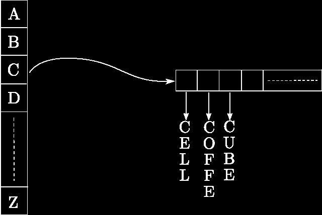
Hash tables are tables (duh! ;)) that are indexed by a hashing value. Generally, in each cell of the table there is a list of items which have properties relative to the hash value. Dictionaries are a good example, if you consider a 26 entry table (Latin alphabet), the hash value will be a letter. For example, 'c', then in the cell corresponding to 'c' you will find all the words beginning by 'c' (see figure 1). Pretty smart isn't it? Of course you can have hash tables in hash tables in hash ...
Figure 1. Hash table example for a dictionary.
Hash tables and Computer Graphics
How can we use that with particle systems? Or more generally speaking, with computer graphics?
Imagine marble slab, wire netting, or any regular grid. If you look at them, you can see that they subdivide space. If you just could index each one of these cells ... Well, this kind of framework exists, i.e. regular 3D grids or even adaptive ones like octrees. Regular 3D grids subdivide all defined space, even where there is nothing and even where throughout the animation there will never be anything (of course then you can reduce it ...). Octrees subdivide all the defined space, more intelligently using an adaptive scheme, i.e, relative to the objects in the scene. A tree traversal is needed, but this framework is still powerful. But then, can't we just index cells where only particles and triangles stand? and anyway, what's a cell?
Go back in your imagination where you were thinking of marble slab or wire netting. You can see a whole bunch of squares well positioned. Let's call these squares "cells". Now if you put your finger in a cell, you have a freedom of motion inside the cell. When you reach the borders, i.e. a line or a corner, you are about to change to another cell. Let's call these lines "discrete lines" and corners "nodes" (in fact, it doesn't have to be discrete, but it is simpler and better for understanding). Mathematically speaking, discrete numbers are integers like 1, 2, 3, 4, ... They are the nodes in the wire netting. Of course if you are thinking in two dimensions, there are integers in the horizontal and vertical axis. When your finger is moving inside a square, you can regard it as a floating value, which is free to move until it reaches the interval's bound (see figure 2), that is, in one dimension, considering the bounds 7 and 8, your finger is able to take all the values in between (e.g. 7.745, 7.08642, ...). So the intervals' bounds will define the cell (in 2D - square - and 3D - cube or voxel). Any value in it can be referenced by one voxel. So? If we detect a polygon and particles inside the cell, there might be a collision. If particles simulate fluid flow, then neighbors are defined by particles inside the voxel. Then the algorithm's complexity is reduced to O(nh) for collision detection where h is the number of polygons inside the cell (generally h<<m, the total number of triangles) and to O(ng) for neighbor searching where g is the number of fluid particles inside the cell (again generally g<<p). This is good! Of course it's hard to reduce it, because we have to traverse all n particles and have to check collisions with close triangles and exchange properties with close particles. We still haven't discussed how to hash, what to hash and what is the complexity of this table lookup algorithm.
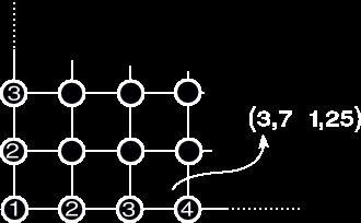
Figure 2. A wire netting.
Hash tables in our case are not specific 3D structures, they are actually the same as the ones used for dictionaries!
Into the concept
So we want cells of a modifiable cell size, we want for each cell to have a list of particles and triangles, we want cells to move since we are dealing with deformable objects, and we want it to operate in O(1), i.e. instantly. Okay ... let's try to do it...
Firstly we are going to hash vertex positions: position as a parameter to a hash function with the cell size (discussed later) will give us a hash value. Into hash_table_entry[hash_value] we insert a reference to the current particle (anyhow you like it best, even a copy) into the list of particles in the voxel (we will see later how this can be optimized). So now we have a list of particles inside a voxel of a cell size defined by the user (which can be modified on the fly by the way). Great, if we are simulating fluids, and want to have neighbor searching, we can simply go throughout this list. And even the list in the 8 neighboring cells if we are talking in 2D or the 26 neighboring cubes if we are talking in 3D (in order to treat the special cases of particles on the border lines or corners). After that we secondly will see how to treat polygons. A little summary:
1. insert all vertices into the hash table.
2. check polygons with the hash table.
3. if polygons and vertices are detected in the same cell*, collision might occur.
*A little foot note here to point out that a vertex belonging to a triangle must not be checked with that triangle (always true)! This algorithm works for collision detection with multiple objects and self intersection too.
Now let's look in the hash tables' machinery.
Hash function and hash value
I have talked about hash function and hash value, without defining them in our case. The hash function will take the particle's position and the cell size as parameters and will return a hash value. This hash value should and will be the same for all the particles inside the same voxel (or square). As I have implicitly said, the hash value is an index of the table, i.e its value is in between 0..table_size. So we need a function that can transform a position, or a bunch of positions, into one unique value. How can this be done? Let's talk in 3D. A position is 3 double, i.e. (x, y, z). Considering a cell size of one, we want the position (1, 1, -1) to be hashed into another cell than the position (-1, 1, 1). We need something unique ... I can't think of anything ... Oh I think I have it ... prime numbers! Yes! If we multiply each component of the position by a different prime number, it will give different values. For the following prime numbers (5, 3, 2), we have
(5 3 2) * (1, 1, -1)' = 6
(5 3 2) * (-1, 1, 1)' = 0
Here I used an additive hash function, i.e. a * x + b * y + c * z. Use what you like most, try and test, for example a good solution is binary operators, i.e. a * x ^ b * y ^ c * z (^ = xor).
The bigger the prime numbers, the better the uniqueness. In fact it happens that different cells (in space) are indexed by the same hash value in the hash table. The algorithm still runs wells, but some useless computations are done. So use big prime numbers. For example 73856093, 19349663, 83492791 to reduce non unique cases. They still happen but can be neglected due to their occasional appearance.
Before computing this function, we must transform the particle's position into the pseudo discrete grid. This is done this way:
        int xd = (int)floor((double)x/cell_size);
        int yd = (int)floor((double)y/cell_size);
        int zd = (int)floor((double)z/cell_size);
Then we can use the following hash function:
unsigned int hash_function(double x, double y, double z, unsigned int cell_size)
{
        int xd = (int)floor((double)x/cell_size);
        int yd = (int)floor((double)y/cell_size);
        int zd = (int)floor((double)z/cell_size);
        return (73856093 * xd + 19349663 * yd + 83492791 * zd)%size;
}
You surely have noticed the modulo size at the end of the return. Size stands for the size of the hash tables. This is in order to keep the hash value in the bounds of the size of the tables. This can be interpreted as a grid of size tables' size that is repeated into space as the hash function respectively is 1, 2, 3, ... the size of the hash table.
Insertion - particles
Once we have the hash value for a particle, in other words a reference to a voxel where the particle stands, we have to insert this particle into a list. This insertion means memory allocation and can be very expensive. Plus for each frame, or each iteration since particles move we have to reallocate the whole hash table. Of course there is a trick to avoid this. The trick here is to use timestamps. At each iteration the timestamps are incremented. When inserting a particle, we insert the timestamps as well. That way in the list, particles that have different timestamps are deprecated. When inserting, we go throughout the list from the beginning to check if there is a deprecated place. If true, replace the deprecated particle with the current one. If not, we insert it. This sort of "head" insertion will be helpful. For example, when checking particles' neighbors, if we find one that has a deprecated timestamps, then the following elements in the list are also deprecated so we do not need to check them (see figure 3). This framework means a lot of allocations in the beginning of the simulations, but still runs fairly well. Also one could simply allocate the lists of the table with the number of particles at the beginning of the simulation (always the trade off between memory consumption and CPU usage).
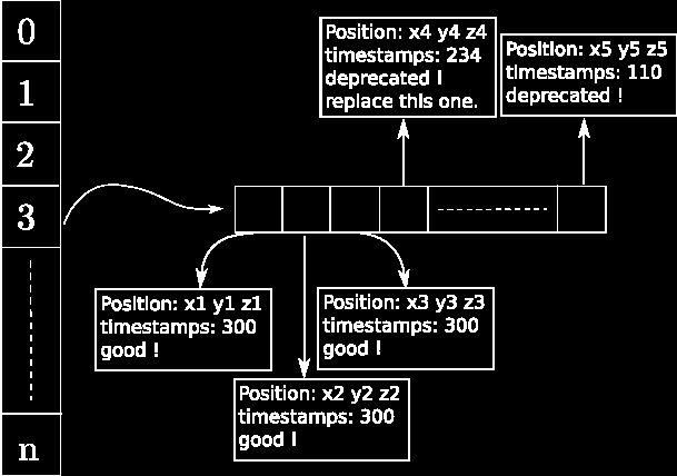
Figure 3. "Head" insertion with current timestamps==300.
When should particles be inserted into the list? Remember the big lines of physical based simulation described above. Instead of parsing all of the objects and all of their particles or vertices after the call of the move function, insertion can be done during this move function. This means giving the hash table as a parameter of the move function. Don't forget to increment the timestamps at the beginning of each iteration. The modified structure is presented a few paragraphs under.
Polygons checking
Once we have hashed all the vertices of all objects, we need to check for collisions. Here we do not take into account edge-edge collisions, but only vertex-triangle. This paragraph will show how the hash table can be used with triangular polygons. Any extension to other kind of mesh is done here. Beware of the special case of self intersections where the vertex belongs to the triangle. Just skip this case.
Our goal is to determine all the cells where the polygons stand, and for each cell detected to check a collision with particles belonging to the cell since collision might occur, with your preferred collision detection and collision response algorithms (see the flipcode tutorial [1] if you are not sure what to do here). Many methods can be employed like AABBox (but not optimized since it is volumetric and our triangle is planar), etc.. Triangular polygons are planar. So we only need to check along the polygons' plane and within the bound of the triangle. Here we propose a scanline algorithm. I call this method rasterization.
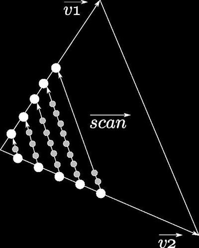
Figure 4. Scanline algorithm.
All that is needed is a timestamp and 3 vertices of the triangle. From these vertices we compute two vectors, v1 and v2, which will be our axis for the scanline. Then for each incrementation, we scan along a new computed vector the cell where we stand and check if collisions might occur (see figure 4). Here is a code snipplet:
bool rasterize(const CPoint3D& p0, const CPoint3D& p1, const CPoint3D& p2)
{
   // define scanline vectors
   CVector3D v1 = (p1-p0) ;
   CVector3D v2 = (p2-p0) ;
   // a check direction vector
   CVector3D v3 = (p2-p1) ;
   double norme1 = v1.getNorme() ;
   double norme2 = v2.getNorme() ;
   // compute the increment step size
   double step_u = (m_cell_size/norme1) - EPSILON ;

   // define starting point in the middle of the starting cell
   int i = (int)floor( (double)(p0.getX()/m_cell_size) ) ;
   int j = (int)floor( (double)(p0.getY()/m_cell_size) ) ;
   int k = (int)floor( (double)(p0.getZ()/m_cell_size) ) ;
   CPoint3D pStart(i+m_cell_size_avg/2.0, j+m_cell_size_avg/2.0, k+m_cell_size_avg/2.0) ;

  // start scanning
  for(double u=0; u<=(1.0+step_u); u+=(step_u))
  {
        CPoint3D pu(p0+u*v1.getPoint());
        CPoint3D pv(p0+u*v2.getPoint());
        // scanning vector
        CVector3D vect_scan(pv-pu) ;
        // check the direction
        if(vect_scan.dotProduct(v3) <0) vect_scan = -vect_scan ;
        pas_scan = (m_cell_size_avg/vect_scan.getNorme())-EPSILON;

        for(double pas_s=0.0; pas_s<=(1.0); pas_s+=(pas_scan))
        {
          tmp = pu+pas_s*vect_scan.getPoint() ;
          // Here you have to "hash" the point tmp to find the hash value of the cell.
          // If this cell has particles with same timestamps, then you have to check for collisions
          // with your favorite algorithm.
        }
  }
}
You probably have noticed a few things. First of all, I use CPoint3D and CVector3D class, which are simple classes of respectively a 3D point and a 3D vector. More importantly, polygons are not inserted into the list. It's just a check. That saves memory consumption! To summarize the whole algorithm, here is how it works:
for each frame
        1) move all objects (i.e. all vertex)
        2) insert all vertices into the hash table
        3) for each polygon check if the cells where they stand are not empty, i.e. possible collisions.
                3.1) if true check for collisions with all the particles into the list
                3.2) if collisions are detected, displace concerned points
Remember that for each frame there can be multiple iterations due to time step restrictions. Generally for collisions the time step is limited to 0.01 (where you should desire 0.04 for 25 images per second), because it is easy to miss a collision if the time step is larger (i.e. the displacement is too big and specially thin objects are missed). Also some physics require small time steps due to arising instabilities.
There are a few issues that should be discussed. Imagine the special case where a polygon is on a border of a cell. There is a vertex next to it, but not in the cell. That means that the vertex is near, might be involved in a collision but is not considered as a colliding point. What should be done in this case is to check the nearby cells of a polygon. Use the normal vector for the height of the polygon. It is true that there are more checks, but when dealing with millions of vertex and polygons, it is worth the case. Also, be very careful with the scanline algorithm, sometimes cells are missed. Maybe more powerful algorithms as the seed feeding should do the job. For any comments or questions about the subject, feel free to email me.
Summary
Here is a code snipplet of the big lines of the physical based simulation algorithm, modified with the hash table steps insertion:
void Scene::moveObjects()
{
        // once and for all
        if (first time)
                compute average length and set the hash tables' cell size

        timestamps++ ;
        // move all objects – remember vertex insertion is done at
        // the end of the move function
        for all objects i  do
        obj[i]->move(step, timestamps, hash_table) ;

        // look out for collisions using the hash table
        for all objects i  do
                obj[i]->rasterization(hash_table) ;
        // remember in this step polygons are "hashed" using the scanline and
        //if vertex and polygons exist in the same cell
        // then collisions might occur. Don't forget the special of
        // a vertex belonging to the polygon ...
}
Hash tables and rendering
There is another thing useful with hash table and space subdivision. For example fluid simulation makes use of particles to compute physics and interactions. But then there are no visible surface, just a bunch of points. So algorithms such as the marching cube can make a surface triangulation out of these particles. How? The utilized space is subdivided into cubic cells (marching tetrahedras make use of tetrahedras). A potential function is called at each of the 8 vertex of the cube; this potential function is computed using the particles in the cell and near this vertex. Having the eight functions computed, we can then define if this voxel is completely filled with a fluid, or completely empty, or is a border. In this last case, triangulation is done using the potential functions. Since it is not the aim of this article I won't go into more details about the marching cube algorithm, but you can find useful information about it on the internet. I will try to write an article on marching cubes on the next Hugi release ... ;).
The good thing is that we don't need to subdivide space for this algorithm, or more precisely we have it already subdivide. We can just reuse the hash table.
Conclusion
There are a few things I need to define before finishing. What are the good values for the cell size and the hash table size? I personally use two hash tables and two different cell sizes. One for the neighboring computations, which is the same used for the marching cube, and one for collision detection. For the neighbor computation, it is relative to the fluids' parameter, so I can't give a numeric value. It should be the size of the attractive and repulsing range. Each fluid particle is then inserted into two hash tables. For the cell size of the hash table used for collision detections, I use the average length of all edges. So I use a preprocessing step before starting simulation which computes the average length. If you use deformable meshes such as mass spring systems, then edges change length. So you are free to recompute this average length, also changing the cell size. It more computationally expensive. I personally don't recompute, just use one preprocessing and it works well.
The hash table size should be around the number of primitives, i.e. the number of vertices plus the number of polygons. The best performance is found using this value. For a more test of different values, you should refer to the article [2]. Actually, almost all that is said here comes from this paper.
I hope you will find some interest reading this article, I just wish this will be useful to you one day. I personally think this method is easy to implement and powerful. One of todays' fastest methods. Of course it can be used for realtime programs (see [2] for time details), it handles self collisions, and useful for neighbor searching and for surface extraction. Any fluid based simulator should use this. Since it is vertex-generic, one can mix multiple meshes such as mass-spring ones, ect.
Even though it took me some time to write this down, I enjoyed it, I find this mag and the demoscene amazingly full of information and creation, thumbs up to both! If you have any questions, don't hesitate to drop a mail.
References
[1] Basic collision detection, Kurt Miller, 2000, link to the article
[2] Optimized Spatial Hashing for Collision Detection of Deformable Objects, Matthias Teschner Bruno Heidelberger Matthias Müller, Danat Pomeranets Markus Gross, Proc. of Vision, Modeling and Visualization, pages 47-54, 2003